The Hilbert curve

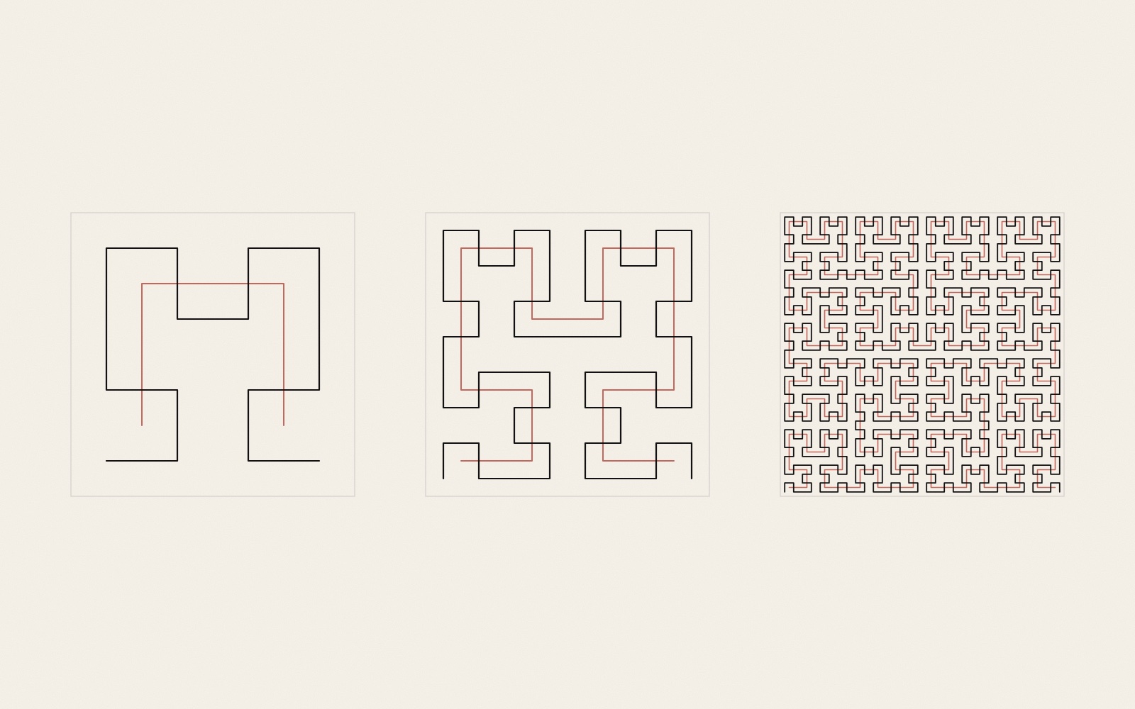
The Hilbert curve is a single path that passes through every cell of a square grid, turning only at right angles and never crossing itself. The German mathematician David Hilbert described it in 1891, a year after Giuseppe Peano had defined the first curve that fills a square.^1, 2

How it is built

Cut the square into four quadrants and join their centres with three lines: up, across, down. That U is the curve of order 1. For order 2, cut each quadrant into four again and put a smaller U in each, turned or mirrored so that the end of one lies next to the start of the next; three short lines join the four copies into one path. Repeat. Brian Hayes, writing in American Scientist, describes it as a program that does not know how to fill a square, but knows that a quarter of a square is also a square, and hands each quarter to itself.¹

Each order has four times as many cells as the one before: 4, 16, 64. After seven orders the path runs through 4⁷ = 16,384 cells.¹ Every finite order is an ordinary line of straight pieces and corners. Only in the limit, after infinitely many subdivisions, does it reach every point of the square.¹

Next order

Peano, Hilbert and the others

Peano gave no picture. He defined two functions that give the x and y of a point in the square for each position along a line. Hilbert simplified the idea and drew it: his paper in Mathematische Annalen has the first published diagram of such a curve, showing its first three stages. Others followed, among them Wacław Sierpiński's curve of 1912, built on triangles, and a closed variant by the American mathematician E. H. Moore, who in 1900 called these objects "crinkly curves".¹

Why near stays near

The useful property is locality: two points close together in the square are usually close together along the curve. Hayes gives an example from Atlanta, where a routing scheme for Meals on Wheels sorted addresses by their position along a Sierpiński curve. On random locations such tours average about 25 per cent longer than the best possible one, found without measuring a single distance.¹ That is the travelling salesman problem, the same one a pen plotter faces when it orders thousands of lines (see plotter path optimisation and TSP art).

The curve is also used to place dots in halftone and dithering, where following it instead of the rows of the image avoids visible line patterns.^1, 3 For a plotter it has one more quality: any order is one unbranched line, drawn from start to end without lifting the pen. See also Plotter Art and Generative Art.

Brian Hayes, whose “Crinkly Curves” is the first source of this note, read it in October 2026 and had nothing to correct. His own interactive explorations of the curve are at bit-player.org.