Contour lines with marching squares

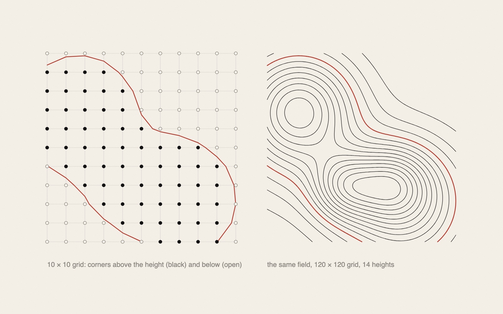
Marching squares is an algorithm that draws contour lines through a grid of measured values, such as heights, temperatures or air pressure. It looks at one small square of the grid at a time, decides from its four corners which of sixteen cases it is, and draws a short line across it; together the short lines form the contours.¹ It is the two-dimensional version of marching cubes, which Lorensen and Cline published in 1987 after research for General Electric on showing CT and MRI scans.²

How it works

Start with values on a grid, for instance heights measured every ten metres, and choose one height, say 50 metres. The contour at 50 metres separates the ground above it from the ground below.

1. Above or below. Mark every grid point 1 if it is above 50 and 0 if it is below.¹
2. Sixteen cases. Take a square of four neighbouring points. Read their four marks in a fixed order, going round the square, as a four-digit binary number. There are sixteen possibilities, from 0000 to 1111.¹
3. The lookup table. A table with sixteen entries says which sides of the square the contour crosses. In case 0000 or 1111 all four corners are on the same side, and nothing is drawn. If one corner is above and three are below, the contour cuts off that corner.^1, 3
4. Where on the side. Without more, every line would cross the sides at their midpoints and the contour would look blocky, made of 45-degree steps.³ Instead the crossing point is found by assuming that the value changes evenly between two corners. If one corner is at 30 metres and the next at 70, the 50-metre line crosses halfway; if they are at 40 and 90, it crosses a fifth of the way from the lower one.^1, 3

Every square is handled on its own, from its four corners and the table.¹ Repeating it for several heights gives a contour map. Lines of one value are called isolines; filled areas between two values are isobands.¹

New drawing

The saddle

Two cases are ambiguous: when diagonally opposite corners are above and the other two below. The contour could then separate the two high corners or join them across the middle. A common answer is to take the average of the four corners as the value at the centre and let that decide.¹ Some programs simply always choose one way.³

Where it is used

Contour lines on topographic maps and isobars on weather maps are the classic uses.¹ In Lund in the 1970s, Mikael Jern's COLOR program was used above all for contour maps, printed in colour on the Hertz ink-jet plotter.⁴ The interview does not say how the contours were computed. In generative art the method draws the contours of a made-up field: the sketch in the note on Perlin noise uses it.

For a pen plotter, the result is thousands of short segments, which have to be joined end to end and put in order before they are drawn; see plotter path optimisation.